SIMD (Single Instruction, Multiple Data)
SIMD
SIMD (Single Instruction, Multiple Data) is a technology that allows a single instruction to perform the same operation on multiple data points simultaneously. In modern processors, SIMD is implemented through specialized registers (e.g., SSE, AVX in Intel processors) that can hold multiple data elements (like integers or floating-point numbers) and execute operations on all elements in parallel. SIMD plays a crucial role in the context of High-Frequency Trading (HFT) by offering notable performance improvements in data processing, which is essential for making rapid trading decisions.
Use of SIMD in HFT
- Data Processing Efficiency: Vectorization: HFT algorithms frequently require real-time processing of substantial volumes of market data. Algorithms may handle several data points (e.g., prices, volumes) simultaneously thanks to SIMD instructions, which cuts down on computation time.
- Algorithm Optimization: Statistical Analysis: SIMD can help huge datasets be handled more effectively by algorithms that carry out statistical analysis, such as volatility computations or correlation analyses between securities. In HFT, moving averages are commonly used to analyze trends in market data. SIMD can accelerate calculations of moving averages by performing simultaneous additions or multiplications across multiple data points.
- Market Data Feeds: Data Feeds Processing: SIMD can enhance the processing of incoming market data feeds, including parsing, filtering, and transforming data formats. This capability is crucial for extracting actionable insights and reacting quickly to market changes.
- Risk Management:
Real-Time Risk Analysis: SIMD aids in real-time risk management by accelerating calculations related to portfolio exposure, risk metrics (e.g., Value-at-Risk), and scenario analysis. This enables traders to make informed decisions swiftly.
Explainer
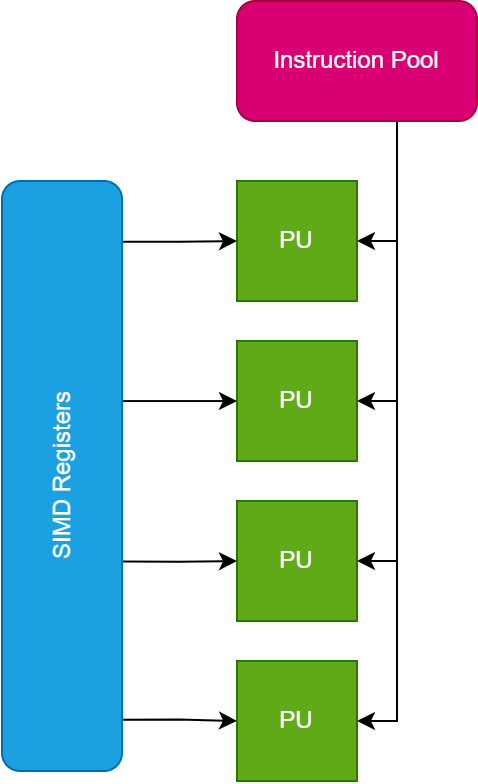
Single Instruction Multiple Data (SIMD) is a parallel computing architecture where a single control unit dispatches the same instruction to multiple processing units simultaneously. Each processing unit then operates on a different set of data. This architecture is particularly effective for tasks that require the same operation to be applied to multiple data points, such as image processing, scientific simulations, and matrix computations. In the provided diagram, instructions are sent from a central source to four processing units. Each processing unit receives the same instruction but processes distinct data inputs, allowing for efficient and simultaneous data processing across multiple units. This parallelism enhances performance by exploiting data-level parallelism within applications. Below is the diagram which explains the architecture for SIMD at CPU level.
Example with Code
Below C++ example calculates a simple moving average. We have two implementations, the first without SIMD and the second with SIMD.
//Function which calculates simple moving average without any SIMD instructions
void calculate_sma_non_simd(const vector<float>& prices, vector<float>& sma, int window_size) {

    size_t size = prices.size();
    for (size_t i = window_size - 1; i < size; ++i) {
        float sum = 0.0f;
        for (size_t j = i - window_size + 1; j <= i; ++j) {
            sum += prices[j];
        }
        sma[i] = sum / window_size;
    }
}
//Function which calculates simple moving average using SIMD instructions
void calculate_sma_simd(const vector<float>& prices, vector<float>& sma, int window_size) {
size_t size = prices.size();
__m256 inv_window_size = _mm256_set1_ps(1.0f / window_size);
for (size_t i = window_size - 1; i + 8 <= size; i += 8) {
__m256 sum_vec = _mm256_setzero_ps();
for (size_t j = 0; j < window_size; ++j) {
__m256 price_vec = _mm256_loadu_ps(&prices[i - window_size + 1 + j]);
sum_vec = _mm256_add_ps(sum_vec, price_vec);
}
__m256 sma_vec = _mm256_mul_ps(sum_vec, inv_window_size);
_mm256_storeu_ps(&sma[i], sma_vec);
}
// Handle the remaining elements
for (size_t i = size - (size % 8); i < size; ++i) {
float sum = 0.0f;
for (size_t j = i - window_size + 1; j <= i; ++j) {
sum += prices[j];
}
sma[i] = sum / window_size;
}
}
Example Run
Assume we have a price vector with 16 elements and a window size of 4:
vector<float> prices = {1, 2, 3, 4, 5, 6, 7, 8, 9, 10, 11, 12, 13, 14, 15, 16};
vector<float> sma(16, 0);
int window_size = 4;
Initial Values • window_size: 4 • inv_window_size: 1.0/4=0.25 , 1.0 / 4 = 0.25, 1.0/4=0.25 • Loop starts at: i = window_size - 1 = 3
Iteration Breakdown First Iteration (i = 3) Initialize sum_vec to zero:
__m256 sum_vec = _mm256_setzero_ps(); // sum_vec = [0, 0, 0, 0, 0, 0, 0, 0]Inner loop to sum up the prices over the window for 8 elements:
for (size_t j = 0; j < window_size; ++j) {
       // load prices[0+j] to prices[7+j]
	__m256 price_vec = _mm256_loadu_ps(&prices[3 - 4 + 1 + j]);
	sum_vec = _mm256_add_ps(sum_vec, price_vec);
}
j = 0: Load prices [1, 2, 3, 4, 5, 6, 7, 8]
__m256 price_vec = _mm256_loadu_ps(&prices[0]); // [1, 2, 3, 4, 5, 6, 7, 8]
sum_vec = _mm256_add_ps(sum_vec, price_vec);  // sum_vec = [1, 2, 3, 4, 5, 6, 7, 8]
j = 1: Load prices [2, 3, 4, 5, 6, 7, 8, 9]
__m256 price_vec = _mm256_loadu_ps(&prices[1]); // [2, 3, 4, 5, 6, 7, 8, 9]
sum_vec = _mm256_add_ps(sum_vec, price_vec);//sum_vec = [3, 5, 7, 9, 11, 13, 15, 17
j = 2: Load prices [3, 4, 5, 6, 7, 8, 9, 10]
__m256 price_vec = _mm256_loadu_ps(&prices[2]); // [3, 4, 5, 6, 7, 8, 9, 10]
sum_vec = _mm256_add_ps(sum_vec, price_vec);  // sum_vec = [6, 9, 12, 15, 18, 21, 24, 27]
j = 3: Load prices [4, 5, 6, 7, 8, 9, 10, 11]
__m256 price_vec = _mm256_loadu_ps(&prices[3]); // [4, 5, 6, 7, 8, 9, 10, 11]
sum_vec = _mm256_add_ps(sum_vec, price_vec);// sum_vec = [10, 14, 18, 22, 26, 30, 34, 38]
Calculate SMA:
__m256 sma_vec = _mm256_mul_ps(sum_vec, inv_window_size); // sma_vec = sum_vec * 0.25 = [2.5, 3.5, 4.5, 5.5, 6.5, 7.5, 8.5, 9.5]Store result in the sma vector:
_mm256_storeu_ps(&sma[3], sma_vec); //sma[3] to sma[10] = [2.5, 3.5, 4.5, 5.5, 6.5, 7.5, 8.5, 9.5]
Results
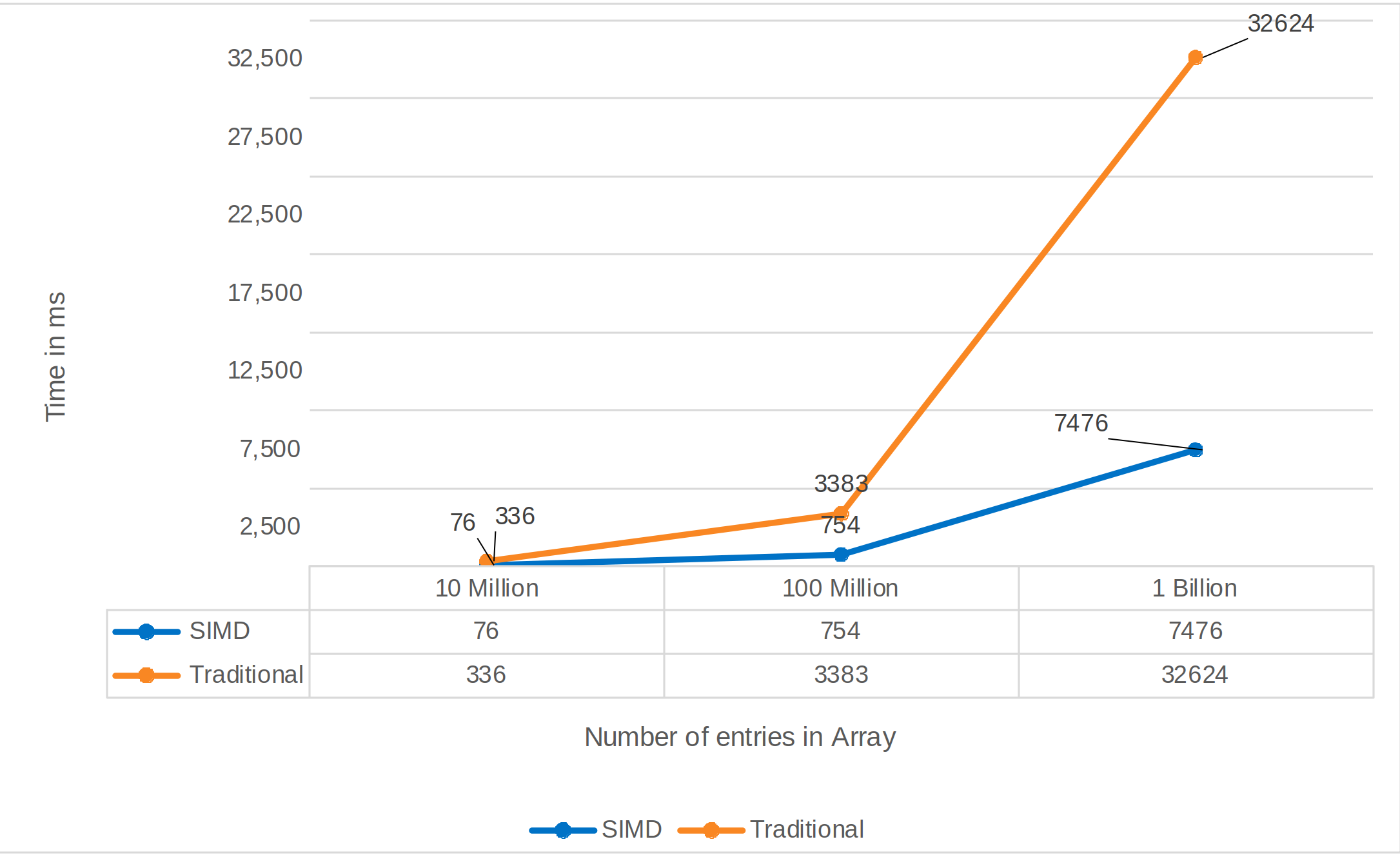
- For the largest array size, the speedup factor is approximately 32624/7476 ≈ 4.36.
- For the medium array size, the speedup factor is approximately 3383/754 ≈ 4.49.
- For the smallest array size, the speedup factor is approximately 336/76 ≈ 4.42.
Conclusion
SIMD instruction is instrumental in HFT for optimizing data processing speed, enhancing algorithm performance, and meeting the stringent low-latency requirements of trading strategies. By leveraging SIMD instructions effectively, HFT firms can gain a competitive edge through faster data analysis, more efficient decision-making, and superior execution capabilities in fast-paced financial markets.